The fractal response
In the first paragraph we have seen how binary logic is in great difficulty in dealing with situations of daily life. Situations where shrinking large quantities in well-defined sets can result in oversimplification of the problem and can lead to paradoxical situations.
In the second paragraph we saw a possible way to overcome the limitations of binary logic by passing through fuzzifing functions that add the appropriate shade to traditional logical categories.
In this section I would like to suggest a field of inquiry that I find personally very suggestive and which, as far as I know, has so far yielded no fruit in the logic in the strict sense. I am talking about fractal geometry.
In the previous examples we have examined cases where the transition between two opposed states occurs gradually. From the grain to the pile, from the haired to the bald, from the warm to the cold etc. In all these cases a fuzzy approach can actually be decisive to grasp the essence of the problem and finally bring the study of the real physical problem into the formal analysis.
But what tools do we have to deal with a case where the transition from the input to the output variables is actually of the “all or nothing” type, with no gradients?
A case so that even when the difference between two values is really small, and even a small alteration of the input value could lead the outright result completely overturn?
In this case, the fading line separating the truth values of our logic it would be so NOT because we admitted the existence of infinite values between the classics 0 and 1, but because we have created a mixture of zeros and ones such that, at some distance, they seem to melt in an indistinct gray. But going to look carefully at the frontier that separates them, it reveals an infinitely complex structure of interwoven truths and falsities.
To visualize this concept I borrow a fractal known as the Newton Fractal. Newton’s fractal is what comes out when representing the basins of attraction in the state space of the dynamic system formed by Newton’s method for solving algebraic equations. This is an iterative method. We want to find the zeros of an algebraic equation: f(x)=0.
Let’s assume a starting value xn and substitute it in the Newton formula that was derived from f(x)
}{f'(x_{n})}")
We get a xn+1 value that will be closer to the roots you searched for than the previous one. We will then replace the value of xn+1 in the Newton formula by repeating the procedure as many times as we consider necessary to reach the root value with the desired precision. The first graphical representation of the Newton method comes from the English mathematician Arthur Cayley. Cayley posed: “Considering all the points of the complex plan as a starting value for the various iterations of the Newton method, to which of the roots of the equation will lead the iteration?” Having three roots, it is reasonable to expect for plan to be divided into three regions, but the real surprise comes out looking at the frontier that separates one from the other. we find that coming from a root area to go to another root, we ALWAYS meet a region that leads to a third root. Obviously this creates a new interface between two other roots and the at transition between these two the same thing occurs, only at a smaller scale.
If we consider the simplest equation,

There are 3 attraction basins and giving the three colors, yellow, green and blue, to the areas that lead to a given root, graphically what comes out is visible in the image below.
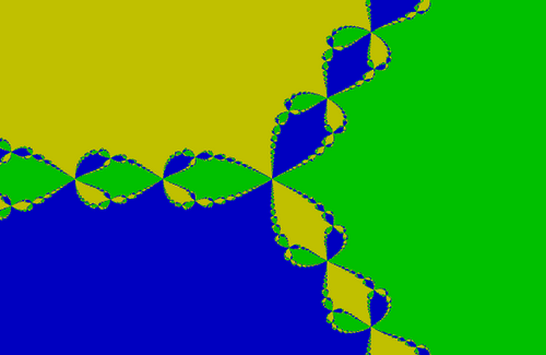
Where we can notice a “drop” shape separating the various regions. And on the border of these “drops” there are other drops and so on to infinity. This is a situation in which two adjoining regions can not coexist without the third region being interposed. If we make a zoom in the previous image, we still find a similar image to the previous one:
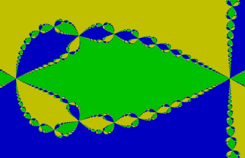
The shape we find is infinitely complex, yet at a certain distance, that is when we have low precision input data, the separation between the areas is very clear.
While Fuzzy logic comes in handy when the border between the sets is blurred, the fractal border tells us what happens varying the accuracy with which we know the values involved in our problem.
 -0
-0  )
)
Leave a Reply